5  Methods

Before we discuss techniques for how to analyze your data, let’s cover a few basic methods that will be useful for all of the example solutions in this book.

5.1 What is a dataframe?

Self-collected data is almost always best represented by a table of the variables you want to study and the values that you collected for each of those variables. The most common type of table is a spreadsheet, which in Personal Science we refer to as a data table or a data frame. Abbreviated “dataframe” or often just “df”, it’s a table of values and variables that always has the same form:

  • columns are variables: the parameters you want to study
  • rows are observations: each incident of data you collected.

It’s important to get in the habit of this row/column approach to data collection because, as you’ll see, all of our tools assume that data will come in a data frame format.

5.1.1 How do I read a dataframe?

Although you are probably used to handling data frames in a spreadsheet program like Excel, in this cookbook we’ll need to start by reading the data into R.

Solution

Use the Tidyverse readr package. Read a CSV-formatted file with the read_csv function. Other Tidyverse let you read many other types of data, including Microsoft Excel (XLSX) files with the function readxl::read_excel().

Regardless of where you get the data, you’ll want to read it into a dataframe. In this case, we’ll save the CSV contents into the dataframe variable headache_df.

Code
library(tidyverse)
headache_df <- readr::read_csv("headache-variables.csv")
headache_df %>% head() %>% knitr::kable()
date headache icecream z wine
2022-07-19 FALSE TRUE 7.557071 0
2022-07-20 FALSE FALSE 7.379434 0
2022-07-21 FALSE FALSE 5.512368 0
2022-07-22 FALSE TRUE 7.600135 0
2022-07-23 FALSE FALSE 8.362155 0
2022-07-24 FALSE FALSE 6.924651 0

Here we peeked at the first 6 lines using the function head() and then sent it to the knitr::kable() function to be printed in this nice format.

5.2 Rolling average

A long series of daily numbers becomes unwieldy after a while, so we’d like to summarize them somehow, perhaps as groups of weeks or months.

Problem You want to take the rolling 7-day average of a series of numbers.

Solution use the rolling() functions in package zoo:

Code
library(zoo)

headache_df %>% 
    mutate(sleep7A = rollapply(z,
                               7, 
                               function(x) {x = mean(x,na.rm = TRUE)},
                               align = 'right',
                               fill = NA)) %>% 
  tail() %>% knitr::kable()
date headache icecream z wine sleep7A
2022-10-19 FALSE FALSE 8.120216 0 6.899738
2022-10-20 FALSE FALSE 5.668099 0 6.738935
2022-10-21 FALSE FALSE 8.093531 0 7.094138
2022-10-22 TRUE FALSE 7.679254 0 7.308210
2022-10-23 FALSE FALSE 7.346326 0 7.283955
2022-10-24 FALSE FALSE 6.019567 2 7.321820

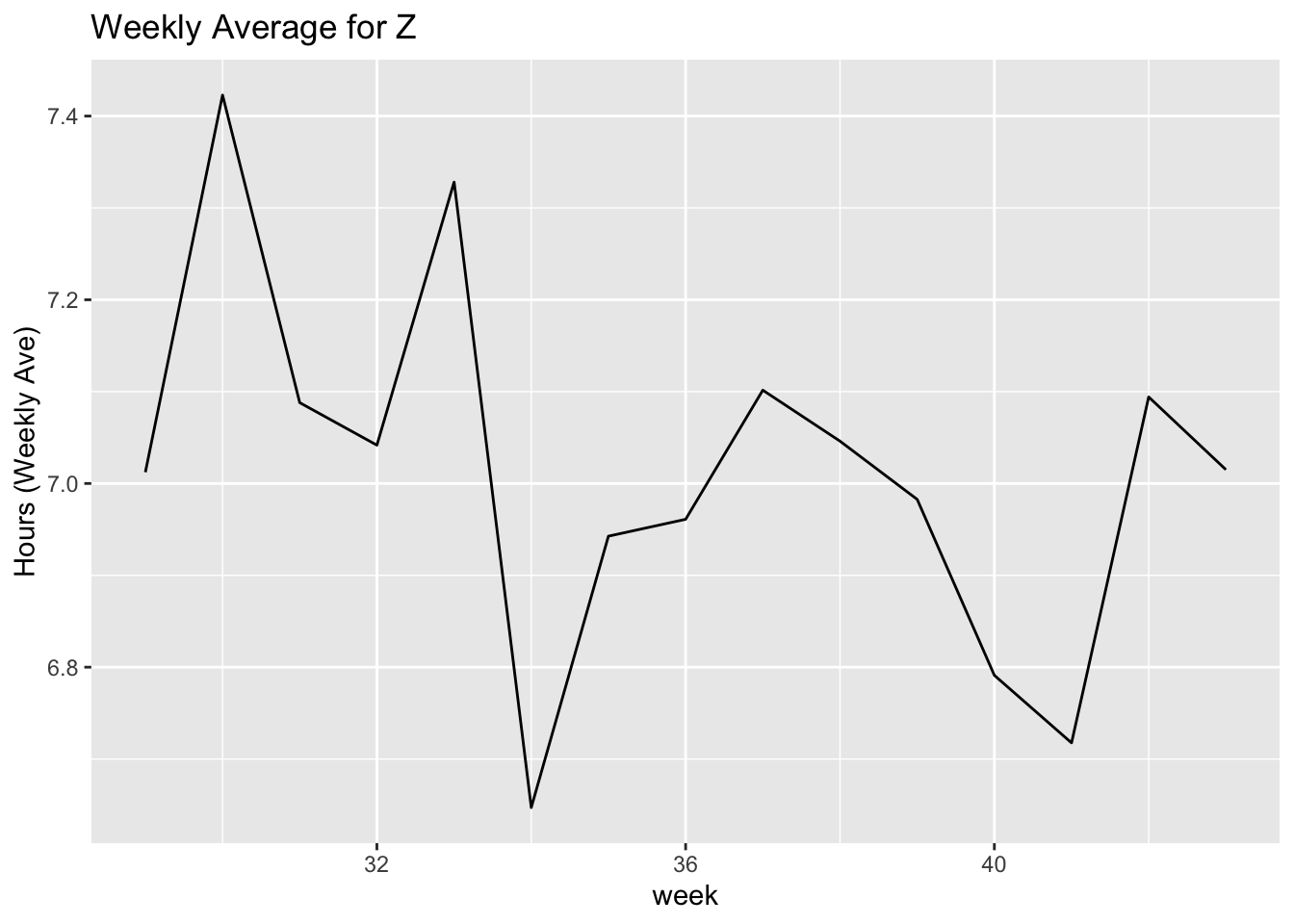
Using the Tidyverse mutate() function, we created a new variable sleep7A to hold the 7-day rolling average for our sleep (Z) variable.

Problem How do we skip the days in between and summarize just the averages by week?

Solution Use summarize().

The Tidyverse function lubridate::week() returns the number of complete seven day periods that have occurred between the date and January 1st, plus one.

Code
headache_weeks <- headache_df %>%
  mutate(week = lubridate::week(date)) %>%
  group_by(week) %>%
  summarize(week_ave = mean(z))

headache_weeks
Code
headache_weeks %>% ggplot(aes(x=week, y = week_ave)) +
  geom_line() +
  labs(title = "Weekly Average for Z", y = "Hours (Weekly Ave)")

5.3 Granger Causality

Problem: Given two sets of time series data, x and y, how likely is it that one series will influence the other.

Solution: see Chicken or the Egg? Granger-Causality for the masses