7  Machine learning

7.1 Multiple regression

When you are tracking lots of variables, it can be difficult to spot exactly which ones are driving an effect.

In this example, we’ve fudged the data so that headaches always happen only on days with less than 6 hours of sleep.

Also, headache days always have high stress. But sometimes we have high stress even without a headache.

Code

library(tidyverse)
library(lubridate)

set.seed(1984)
WEEKS <- 140

z <- function(x){
m = NULL
for(i in 1:WEEKS){
  m = c(c(rep(0,6),
              floor(runif(1,min=0,max=3))),
        m)
}

m
}
tracking_table <- data.frame(date=seq(from = today()-weeks(WEEKS),
                     by = "1 day", length.out = 7*WEEKS),
            headache = sample(c(TRUE,FALSE), 7*WEEKS,
                              prob = c(.05,.95),
                              replace = TRUE),
            stress = sample(c("low","medium","high"),
                            size = 7*WEEKS,
                            replace = TRUE),        
            icecream = sample(c(TRUE,FALSE), 7*WEEKS,
                              prob = c(.10,.90),
                              replace = TRUE),
            z = runif(7*WEEKS, min = -2.5, max = .5) + 8,
            wine = z(0))

tracking_table$headache <- tracking_table$z<6  # make headaches on days with low sleep
# tracking_table[tracking_table$stress=="high"] <- "high"  # make stress on headache days

knitr::kable( head(tracking_table,10), digits = 2) %>%
  kableExtra::kable_styling(bootstrap_options = c("striped", "hover", "condensed"))

date	headache	stress	icecream	z	wine
2020-04-15	FALSE	high	FALSE	8.24	0
2020-04-16	FALSE	high	FALSE	6.60	0
2020-04-17	FALSE	medium	TRUE	7.16	0
2020-04-18	FALSE	low	FALSE	6.89	0
2020-04-19	FALSE	high	FALSE	6.04	0
2020-04-20	FALSE	high	FALSE	7.34	0
2020-04-21	TRUE	high	FALSE	5.74	0
2020-04-22	FALSE	high	FALSE	6.87	0
2020-04-23	FALSE	low	FALSE	7.23	0
2020-04-24	FALSE	high	FALSE	6.89	0

Now make a linear model using the 980 rows from our dataframe.

Code

m <- lm(headache~icecream+z+wine+stress, data = tracking_table)
summary(m)

Call:
lm(formula = headache ~ icecream + z + wine + stress, data = tracking_table)

Residuals:
     Min       1Q   Median       3Q      Max 
-0.46762 -0.21394 -0.03199  0.16852  0.57443 

Coefficients:
              Estimate Std. Error t value Pr(>|t|)    
(Intercept)   2.085871   0.073447  28.400   <2e-16 ***
icecreamTRUE  0.030793   0.028976   1.063    0.288    
z            -0.272406   0.010301 -26.445   <2e-16 ***
wine         -0.002729   0.019588  -0.139    0.889    
stresslow    -0.012375   0.022061  -0.561    0.575    
stressmedium -0.034324   0.021410  -1.603    0.109    
---
Signif. codes:  0 '***' 0.001 '**' 0.01 '*' 0.05 '.' 0.1 ' ' 1

Residual standard error: 0.2776 on 974 degrees of freedom
Multiple R-squared:  0.4216,    Adjusted R-squared:  0.4186 
F-statistic:   142 on 5 and 974 DF,  p-value: < 2.2e-16

Those triple dots (“***”) in the right-hand column for Coefficients indicate items of very high significance.

In this case, as expected, there seems to be a strong relationship between both sleep and stress.

A quick yet dramatic way to visualize this uses the stat_smooth function of ggplot:

Code

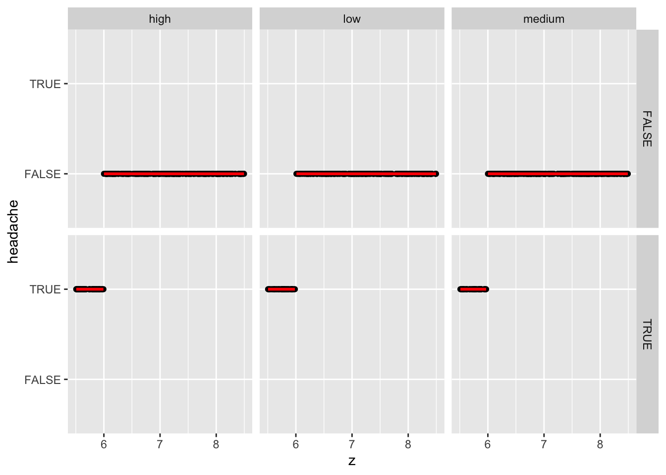
tracking_table %>% ggplot(aes(y=headache, x=z)) + geom_point() + stat_smooth(formula = y~x, method = "lm", color = "red") +
facet_grid(headache ~ stress)

We clearly see that headaches always occur on days when Z<6.

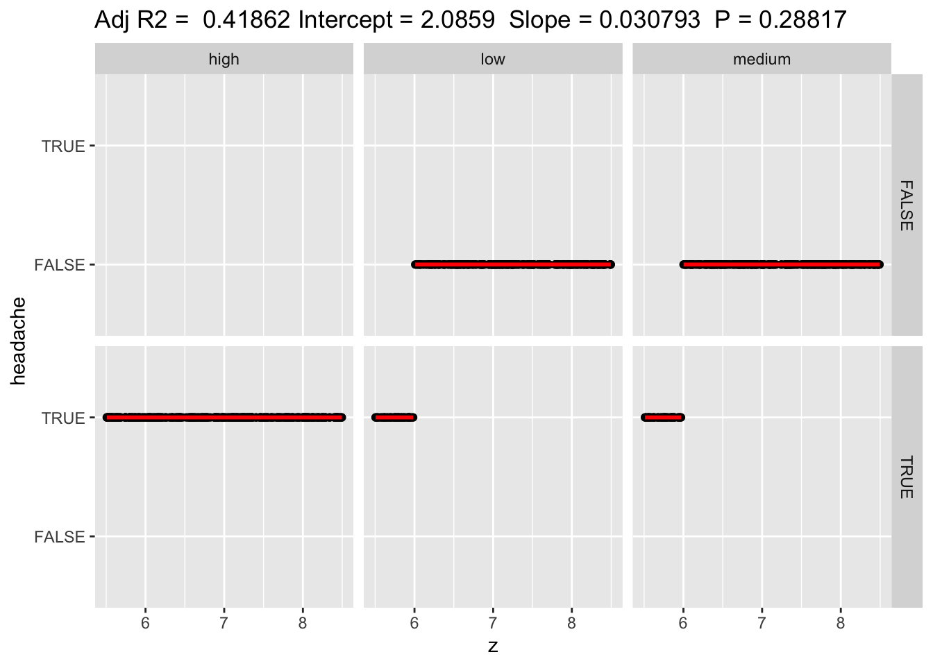
And here’s what happens if we change the data so headaches always happen when stress is high.

Code

tracking_table[tracking_table$stress == "high",]$headache <- TRUE

tracking_table %>% ggplot(aes(y=headache, x=z)) + geom_point() + stat_smooth(formula = y~x, method = "lm", color = "red") +
facet_grid(headache ~ . + stress) +
  labs(title = paste("Adj R2 = ",signif(summary(m)$adj.r.squared, 5),
                     "Intercept =",signif(m$coef[[1]],5 ),
                     " Slope =",signif(m$coef[[2]], 5),
                     " P =",signif(summary(m)$coef[2,4], 5)))

As expected, the plot shows headaches either when z<6 or when stress is high.