10  Averages vs n-of-1

10.1 Averages vs N-of-1

Consider the following case:

1000 people took Vitamin D for 6 months. We measured their Vitamin D levels before and after, and sure enough: the average levels after are higher than before.

More specifically, let’s say the average at the beginning of the study is 30 mg/nL, widely considered the absolute minimum for a healthy person.

Code

study <- tibble(subject=1:N,
                vitamind=rnorm(n=N,
                               mean=MEAN_VITAMIN_D,
                               sd=MEAN_VITAMIN_D
                )
                ) %>% 
  transmute(subject, vitamind=if_else(vitamind<0, 0,vitamind))

study_plot <- study %>% ggplot(aes(x=subject,y=vitamind)) + 
  geom_point() +
  geom_smooth(method= lm, formula= y ~ x, color="red") + 
  labs(x="Subject", y = "Vitamin D (ng/mL)", title = "Vitamin D levels in all subjects")

study_plot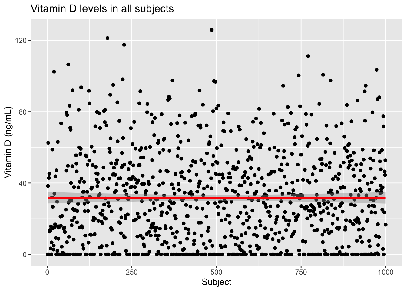

Red line indicates the average slope of the points

Note that, although the average level is about 30 mg/mL, there are many subjects whose levels are considerable above and below that.

Code

maxd <- max(study$vitamind)
study_plot + 
  geom_rect(xmin=0,ymin=0,xmax=N, ymax=MEAN_VITAMIN_D - sd(1:MEAN_VITAMIN_D),
            fill = "lightblue",
            alpha = 0.007) +
    geom_rect(xmin=0,ymin=MEAN_VITAMIN_D + sd(1:MEAN_VITAMIN_D),xmax=N, ymax=maxd,
            fill = "lightblue",
            alpha = 0.007)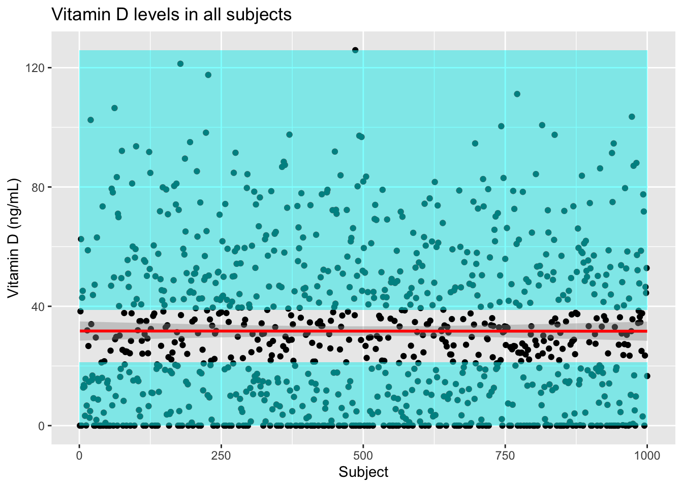 

Shaded area represents points more than a standard deviation outlier.

Another way to represent the study is with a boxplot variation called a violin plot.

Code

study %>% ggplot() + 
  geom_violin(aes(x=subject,y=vitamind),
              draw_quantiles = c(0.25, 0.5, 0.75)) + 
  labs(x="", y = "Vitamin D (ng/mL)", title = "Vitamin D levels in all subjects")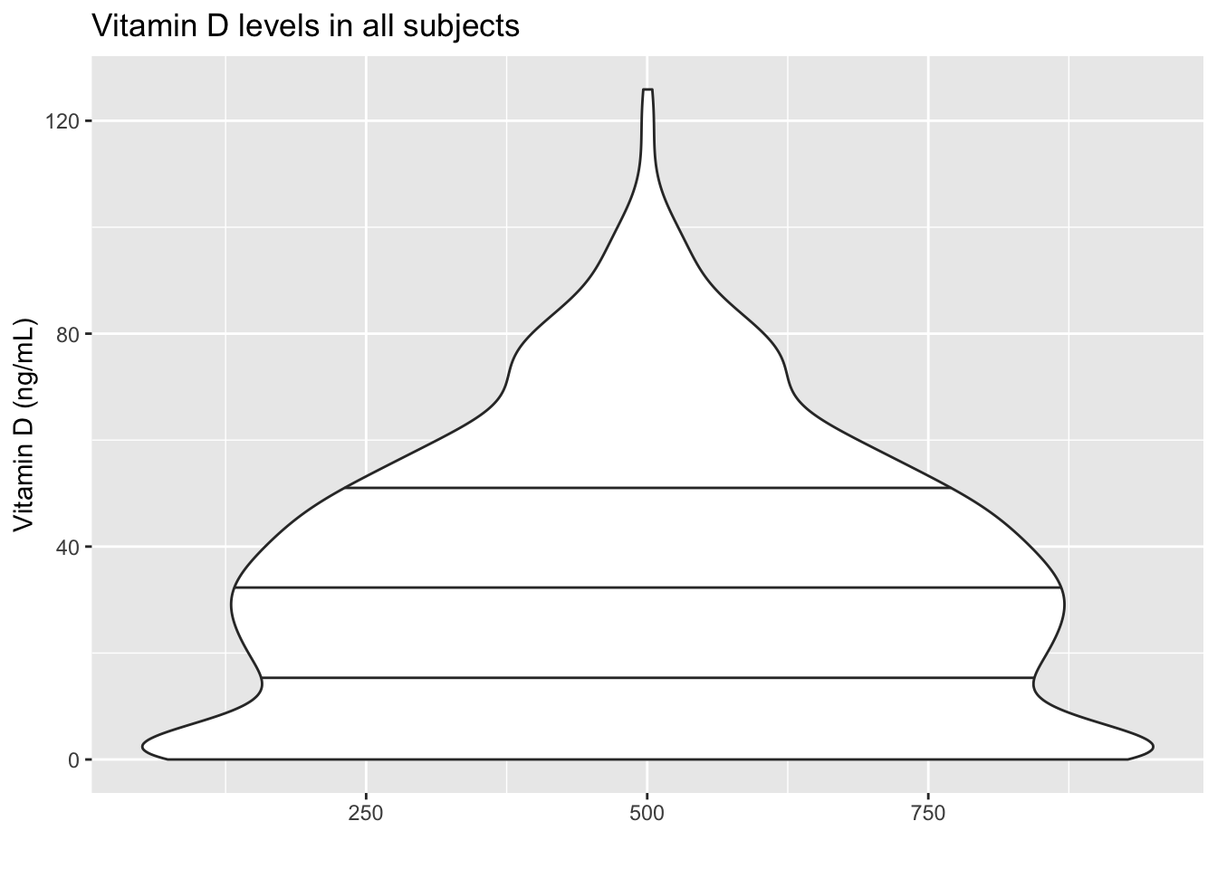

The width of this plot shows the proportion of subjects at particular Vitamin D levels. (The horizontal lines indicate the different quartiles of the data)

To make this more fun, let’s assume we have additional information about the subjects in our trial.

Code

study <- cbind(study,
 nationality = replicate(N, sample(c("USA","Japan","Europe"),size=1)),
 weight = rnorm(n=N, mean = 120, sd = 50))